Analysis operators

Label operators

clean-borders [-l]

This operator removes the image contents touching the borders. This is obtained by subtracting from the input image its morphological reconstruction from the border. The operator can be applied to both intensity and label images; however, its typical application is the removal of segmented objects that intersect the image border.

The -l option must be used when processing label images.

click-select [-d max-distance] <positions.vx>

This operator selects labels in the input image based on specified positions. The algorithm works by determining for each position the closest label, i.e. the label having the pixel/voxel closest to the specified position. Proximity is measured using Euclidean distance, taking into account the spatial calibration of the image.

The file <positions.vx> contains the positions to be used for the selection, following the sviewer in-house shape file format. The positions should be defined in the physical space of the image.

The -d option allows to set a maximum distance, above which labels are simply ignored.

click-replace [-d max-distance] <positions.vx> <new-value>

This operator replace labels in the input image based on specified positions. The algorithm works by determining for each position the closest label, i.e. the label having the pixel/voxel closest to the specified position, and replaces this label by a new value. Proximity is measured using Euclidean distance, taking into account the spatial calibration of the image.

The file <positions.vx> contains the positions to be used for the selection, following the sviewer in-house shape file format. The positions should be defined in the physical space of the image. The parameter <new-value> specifies the value to assign to the selected labels.

The -d option allows to set a maximum distance, above which labels are simply ignored.

label-boundaries [-a]

This operator computes the boundaries between labels in an image. By default, the output is a binary image of the boundaries. If the -a option is specified, the boundaries are overlaid to the labels of the input image.

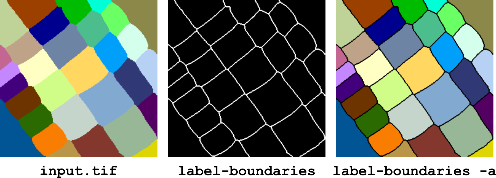
Figure 7 Computing boundaries between labels with label-boundaries.

label-defragmentation [-n 4,6|8,26]

This operator takes as input a label image in which each label may appear as several connected components. The operator retains the largest component for each label and removes all the other ones. The discarded components are removed by filling the holes they make in the largest components of other labels.

The connectivity used to define connected sets is set with the -n option. See Neighbourhood systems and connectivity for more information about the meaning and usage of this option.

replace largest|<label>[,<label2>,...,<labelN>] <value>

This operator replaces one or several label values in an image by the specified value. Several values to be replaced can be specified using a comma-separated list of values. The ’-’ character can be used to specify label ranges in the list. For example:

bip replace 17,19-21,largest,37 0 image.tif

replaces all occurrences of labels 17, 19, 20, 21, 37 plus the most represented label by 0.

The keyword largest can be used anywhere in the list to refer to the label that is the most represented in the image. Remind that 0 is not considered as a label value, which implies that the background cannot be selected as the largest label.

select [-r <range>] largest|max|<label>[,<label2>,...,<labelN>]

This operator selects one or several labels in an image. All values not appearing in the specified list are set to 0. The values of the listed labels are left unchanged.

The option -r can be used to set the range of neighbours to be included in the selection. For example, specifying -r 1 also includes in the selection all the immediate neighbours of the specified labels. Only first-order neighbourhood is supported in the current implementation.

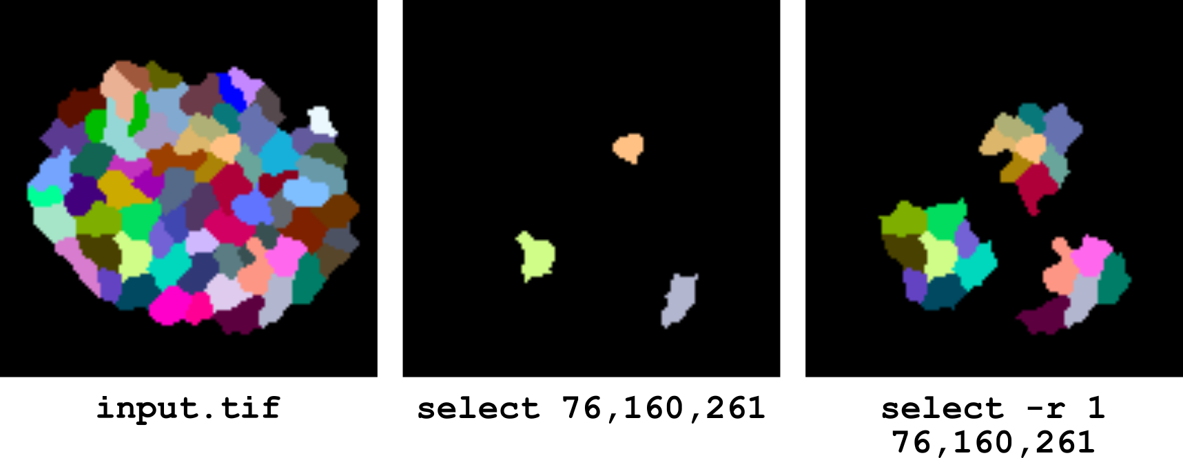
Figure 8 Selection of labels and of their immediate neighbours.

The keyword max can be used anywhere in the list to refer to the label with the largest value in the image.

Similarly, the keyword largest can be used anywhere in the list to refer to the label that is the most represented in the image. Remind that 0 is not considered as a label value, which implies that the background cannot be selected as the largest label.

To select the background of a label image (i.e., to obtain a binary mask of the background alone), one should use for example the following pipeline:

bip pipeline -e "threshold 1 | invert auto" image.tif

select-fringe

This operator selects the labels located at the fringes in a segmented image. A label is a fringe label if the graph of its neighbours is not cyclic. Note that this is not systematically the same as outer labels (labels having contacts with the background). Outer labels are not necessarily fringe labels. Conversely, fringe labels will generally be outer labels, but there are rare configurations where they may not.

In practice, users will probably need the select-outer operator for most applications. The select-fringe operator will be particularly useful to select the outer rim of a cell layer in 3D.

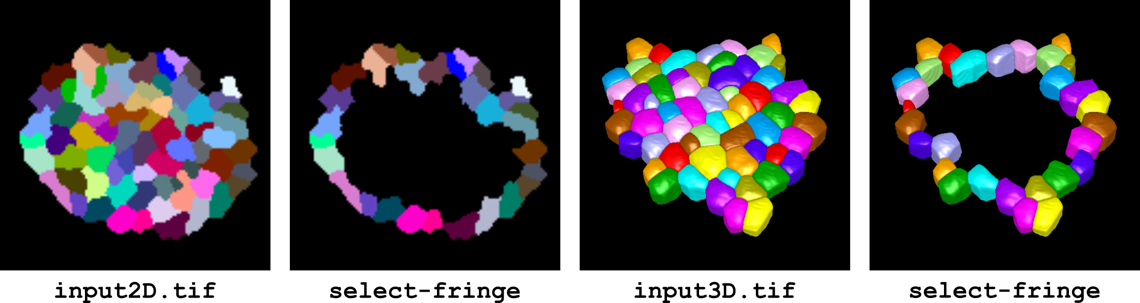
Figure 9 Selection of fringe labels in 2 and 3 dimensions.

select-inner

This operator selects the inner labels in a segmentation. A label is an inner label if it is not in contact with the image background. The set of obtained labels is the complement of those obtained with operator select-outer.

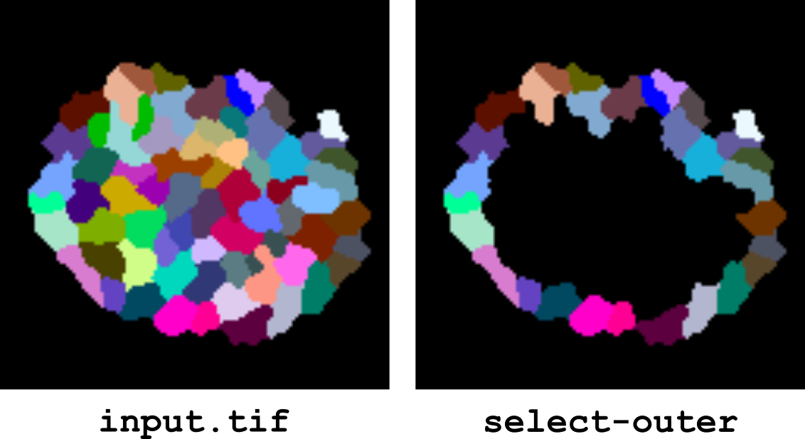
select-outer

This operator selects the outer labels in a segmentation. A label is an outer label if it contacts the image background. Note that this is not systematically the same as fringe labels. Outer labels are not necessarily fringe labels. Conversely, fringe labels will generally be outer labels, but there are rare configurations where they may not.

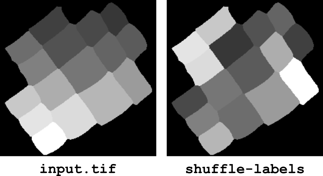
shuffle-labels

This operator randomly shuffles the label values in an image. The background (label value 0) is left unchanged. This operator is for example useful to modify the contrast at the boundaries between the labeled objects (both when displaying labels as gray levels or as false colors).

split [-h <tolerance>]

This operator separates objects that are touching each other in a binary image. The optional tolerance parameter can be set to control the degree of separation (default tolerance value is 0.5). The higher the tolerance, the less the objects are split (Figure 10).

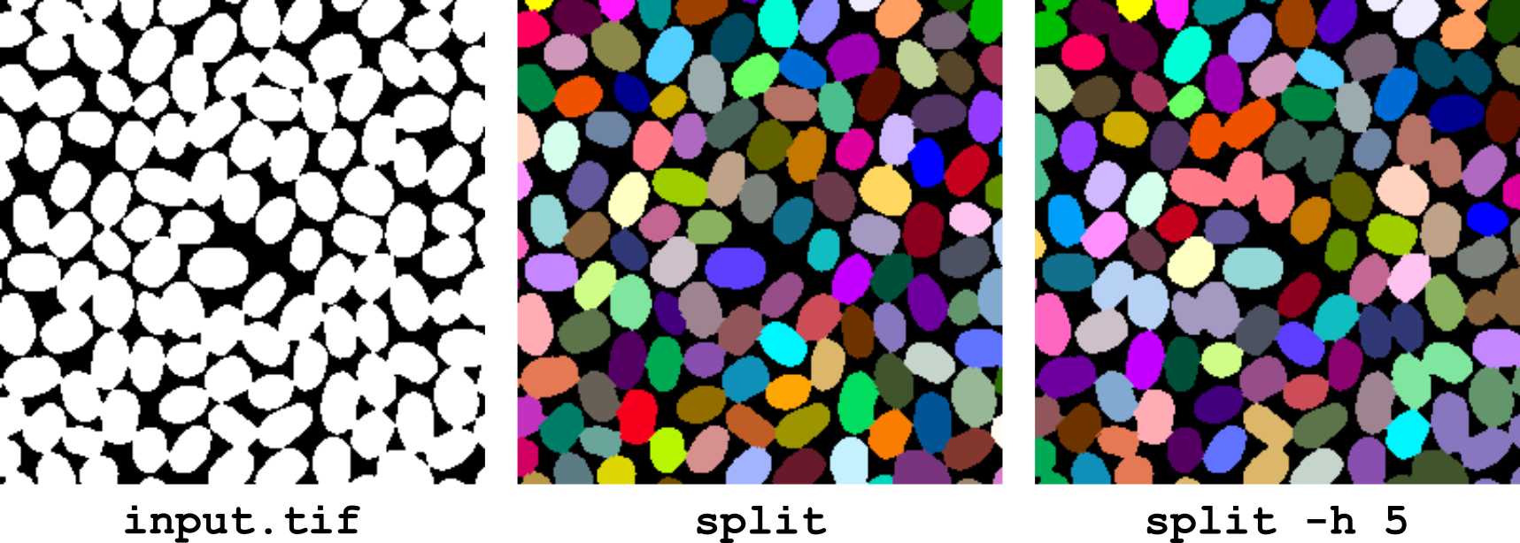
Figure 10 Separating touching objects using the split operator.

The split operator can also process label images of segmented objects. In this case, the original labelling is lost because a thresholding of values above 0 is applied as a first step in this operator.

swap-labels <list1> <list2>

This operator swaps values in an image. The values to swap are specified by two lists of comma-separated values. The two lists must have the same size. All image positions having a value from list1 are assigned the corresponding value in list2, and reciprocally.

zmap [-l]

This operator performs a Z-front detection in the input 3D label image. Z-front detection is a 2D projection of the 3D image: at each XY position, it determines and retains the first Z position with a non-null value. Used in conjunction with the reverse operator izmap, this operator is typically used to extract the uppermost layer in a label image.

If the -l option is set (“label mode”), then the operator retains the first encountered label rather than its Z position.

Distance maps

chamfer-distance <foreground>

This operator computes an integer-valued map of the approximate distance between each image position and the closest position with value foreground. The input image is not necessarily binary, as every non-foreground position will be considered as background. The implementation follows algorithms given by Borgefors [Borgefors, 1986, Borgefors, 1996].

This operator is provided for historical and pedagogical reasons. Users will in general opt instead for the Euclidean distance operator, which is very efficient and provides exact distance values.

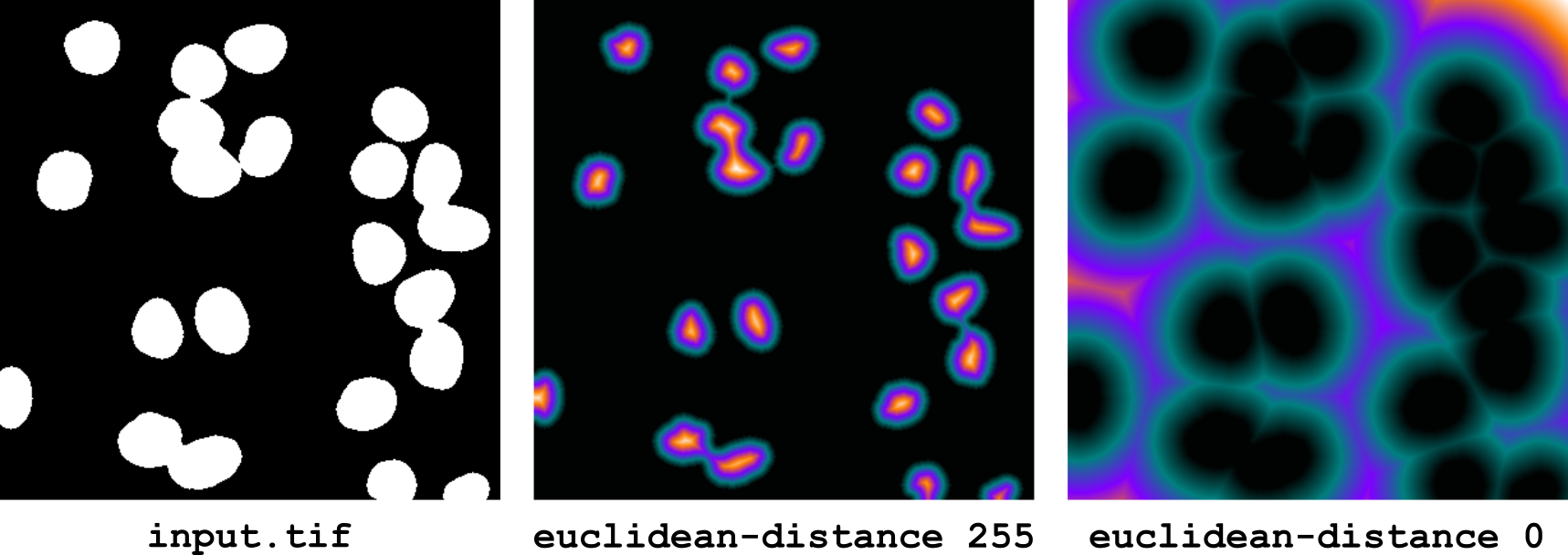
euclidean-distance [--physical] <foreground>

This operator computes a real-valued map of the exact Euclidean distance between each image position and the closest position with value foreground. The input image is not necessarily binary, as every non-foreground position will be considered as background. The implementation is based on Felzenszwalb and Huttenlocher’s algorithm [Felzenszwalb and Huttenlocher, 2012] that we have modified to take into account the spatial calibration of the image.

By default, the distance is computed in pixels (2D) or voxels (3D). If the --physical option is set, the distance is instead computed in physical units, taking into account the spatial calibration of the image and its anisotropy, if any.

The numerical type of the output image is 32-bit floating point.

Measurements

intensity-analysis [-b <boundary>] [-p <parameters>] [-o <output.tsv>] [-s] <intensity-path>

This operator performs intensity measurements on objects in a segmented image. Each label in the input image defines an object. In practice, an object will generally correspond to a unique connect component in the input label image, but BIP imposes no restriction on the number of components per object.

For each input image, the measurements are performed on the paired image specified by intensity-path. This path can be either a path to a single filename or a directory name. In the second case, BIP will look in the specified directory for a file matching the input filename. Modifiers can be used to pair images with systematic differences in their filenames. See Pairing images by matching filenames to learn more about pairing images.

Example 1. Assume we have the following organization of project files, with separate directories for intensities and labels, but identical filenames for each image pair:

project/
  raw/
    image1.tif
    image2.tif
    image3.tif
  labels/
    image1.tif
    image2.tif
    image3.tif
  results/

Then, from the results directory, intensity analysis can be invoked as:

bip intensity-analysis ../raw ../labels/*.tif

Example 2. Assume we have instead different filenames for intensities and labels:

project/
  raw/
    image1.tif
    image2.tif
    image3.tif
  labels/
    labels1.tif
    labels2.tif
    labels3.tif
  results/

Then intensity analysis would be invoked using a pattern substitution:

bip intensity-analysis ../raw:s/labels/image/ ../labels/*.tif

Explicit boundary value. By default, it is assumed there is no specific label for the boundaries between objects. This corresponds to the situation where different object labels may be in contact. If a specific label has been used to label boundaries at the segmentation stage (as done for example when computing the dams in a watershed transform), then this value must be specified using the -b option.

Parameter selection. By default, BIP performs measurements for all available intensity parameters (Table 3). This behaviour can be overridden by using the -p option to specify a comma-separated list of desired parameters. For example, the following call will only measure the average and median intensity within each object:

bip intensity-analyis -p mean,median ../raw ../labels/*.tif

Table 3 Intensity measurements available in BIP.

Parameter	Definition
sum	Sum of intensity values
mean	Average of intensity values
median	Median of intensity values
min	Minimum intensity value
max	Maximum intensity value
stddev	Standard-deviation of intensity values
mad	Median of absolute deviation of intensity values

Output files. On output, BIP writes a intensity-analysis.tsv text file, which obeys the TSV format (columns of measured values separated by tabulations). This file can be loaded in software such as Excel, LibreOffice Calc, gnuplot, or R for downstream statistical analysis and graphical plotting. The name of the output file can be changed using the -o option.

If the -s option (“split”) is set, BIP will instead save the measurements in a different file for each input image. The output files are named from the basenames of the input files (<basename>.tsv). In this mode, the -o option is ignored.

region-analysis [-p <parameters>][-b <boundary-value>]

This operator performs quantitative measurements on objects in a labelled image. Each label in the input image is considered as defining an object. In practice, an object will generally correspond to a unique connected component in the input label image, but BIP imposes no restriction on the number of components per object.

By default, it is assumed there is no specific label for the boundaries between objects. This corresponds to the situation when different object labels may be in contact. If a specific label has been used to label boundaries at the segmentation stage (as done for example when computing the dams in a watershed transform), then this value must be specified using the -b option.

By default, BIP performs measurements for a large number of parameters. This behaviour can be overridden by using the -p option to specify a comma-separated list of desired parameters. For example, the following call will only measure the number of voxels, the volume and the sphericity of objects in a 3D image:

bip region-analyis -p count,volume,sphericity image3D.tif

Available parameters in BIP fall into one out of three categories. Most parameters are simple parameters, for which a single numerical value is obtained (e.g., area). Table 4 lists the available simple parameters. Some other parameters are vector parameters, which provide several values corresponding to as many simple parameters that are components of a vector (such as a position or a direction). One example is the centroid parameter, which provides on output 2 or 3 parameters (centroid-x, centroid-y and centroid-z), corresponding to the coordinates of the average position of an object. Lastly, group parameters are short-cuts for specifying groups of related simple or vector parameters, without having to specify each parameter individually. For example, asking for the size parameter triggers the measurements of the count, area, and volume parameters. Table 5 lists the available vector and group parameters.

Table 4 Simple parameters available in BIP. Dimension indicates in which dimension(s) each parameter is defined. Parameters not defined for a given dimension will appear as NaN in the measurement file.

Parameter	Definition	Dimension
Size measurements
area	Object area in physical units	2D
count	Number of pixels (2D) or voxels (3D)	2D,3D
volume	Object volume in physical units	3D
equiv-radius	Radius of disk (or sphere) of same area (volume)	2D,3D
major-radius	Radius along the first principal axis	2D,3D
medium-radius	Radius along the 2nd principal axis	3D
minor-radius	Radius along the smallest principal axis	2D,3D
gyration-radius	Root mean squared distance to object centroid	2D,3D
perimeter	Length of the object boundary	2D
surface-area	Surface area of the object boundary	3D
box-diagonal	Diagonal of the axis-aligned bounding box	2D,3D
Position measurements
centroid-x	Centroid: x-coordinate	2D,3D
centroid-y	Centroid: y-coordinate	2D,3D
centroid-z	Centroid: z-coordinate	3D
box-x1	Axis-aligned bounding box: x-coordinate of 1st corner	2D,3D
box-y1	Axis-aligned bounding box: y-coordinate of 1st corner	2D,3D
box-z1	Axis-aligned bounding box: z-coordinate of 1st corner	3D
box-x2	Axis-aligned bounding box: x-coordinate of 2nd corner	2D,3D
box-y2	Axis-aligned bounding box: y-coordinate of 2nd corner	2D,3D
box-z2	Axis-aligned bounding box: z-coordinate of 2nd corner	3D
Orientation measurements
major-vector-x	Largest principal axis: x-coordinate	2D,3D
major-vector-y	Largest principal axis: y-coordinate	2D,3D
major-vector-z	Largest principal axis: z-coordinate	3D
minor-vector-x	Smallest principal axis: x-coordinate	2D,3D
minor-vector-y	Smallest principal axis: y-coordinate	2D,3D
minor-vector-z	Smallest principal axis: z-coordinate	3D
medium-vector-x	Intermediate principal axis: x-coordinate	3D
medium-vector-y	Intermediate principal axis: y-coordinate	3D
medium-vector-z	Intermediate principal axis: z-coordinate	3D
Shape measurements
elongation	Length-ratio between largest and intermediate axes	2D,3D
flatness	Length-ratio between intermediate and smallest axes	3D
circularity	Matching with a disk having the same area	2D
sphericity	Matching with a sphere having the same volume	3D
globularity	(Experimental)	2D,3D
Topological measurements
degree	Number of neighbouring labels	2D,3D
outer	Indicator of contact with the background	2D,3D
fringe	Indicator of localization at the periphery of the tissue	2D,3D
layer	Number of the containing tissue layer	2D,3D

Table 5 Vector and meta-parameters available in BIP.

Parameter	Definition	Associated simple parameters
centroid	Object average position	centroid-x, centroid-y, centroid-z
size	Object size	count, area, volume
box	Axis-aligned bounding box	box-x1, box-y1, box-z1, box-x2, box-y2, box-z2, box-diagonal

On output, BIP writes a region-analysis.tsv file, which obeys a TSV format (columns of measured values separated by tabulations). This file can be loaded in software such as Excel, LibreOffice Calc, gnuplot, or R for downstream statistical analysis and graphical plotting.

As a for most BIP operators, both 2D and 3D images can be passed upon a same call to the region-analysis operator. Some parameters are defined in both 2 and 3 dimensions (such as count, the number of times the label is observed in the image), while others are specific to either the 2D (such as area) or the 3D case (such as volume). BIP reports a NaN (not-a-number) value in the output file for undefined parameters.

Images with multiple channels and/or multiple timepoints can be passed to the operator, in which case labelled regions will be quantified in the different channels and time frames. A channel column is added in the output file in case the input image contains several channels. Similarly, a timepoint column is added in the output file in case the input image contains several timepoints. Images with different numbers of channels or timepoints can be mixed during a same call.

Export operators

export-bboxes

This operator computes the bounding boxes of the labelled regions in the input image. The coordinates of the bounding boxes are expressed in the physical space (i.e., taking into account the spatial calibration of the image). For each label, the corresponding box is stored in a file named by appending the label to the input filename. The channel and the timepoint are also added to the filename if the input image contains several channels or timepoints. The output file format is Free-D’s shape viewer format.

export-shapes [--stl]

This operator computes the triangular meshes corresponding to the boundaries of labelled regions in a 3D image. One mesh is computed for each label and stored in a file named by appending the label to the input image filename. The mesh is obtained by applying the Marching Cubes algorithm [Lorensen and Cline, 1987] to the binary mask of the label.

The default output file format is an in-house shape file format (.tm files) suitable for loading and display with sviewer, the Free-D’s standalone 3D shape viewer [Biot et al., 2016].

You can switch to the STL file format using the --stl option.

export-rag

This operator computes the region adjacency graph (RAG) of the input image. In the RAG, each labelled region of the input image is represented by a node placed at the centroid (geometrical center) of the region. The nodes that correspond to neighbouring regions are connected by edges.

The computed RAG is stored in a format (file with extension .cs) suitable for opening with sviewer, the Free-D’s standalone 3D shape viewer [Biot et al., 2016]. A typical sequence of operations to compute and display the RAG is thus:

bip export-rag image3D.tif
sviewer image3D-rag.cs

See Figure 11 for a typical example of 3D display.

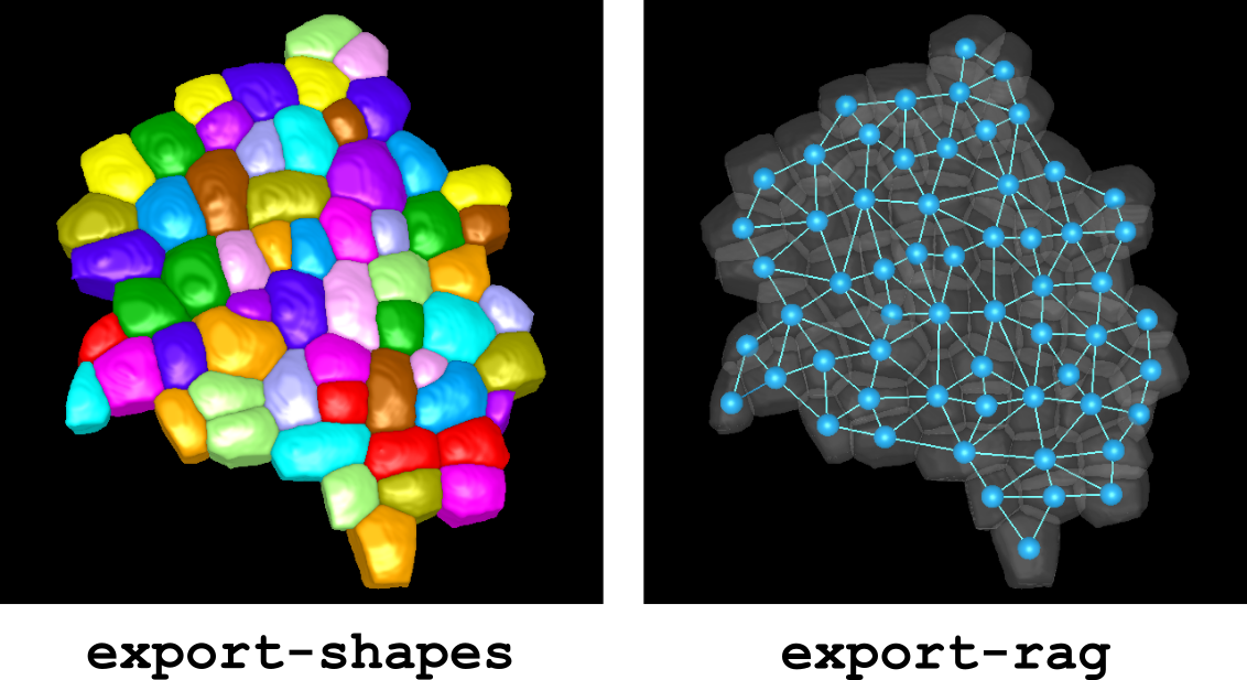
Figure 11 Exporting and displaying shapes and RAG in a 3D label image.