Tutorials
The examples below illustrate how diverse tasks of varying complexity can be performed by combining BIP operators (typically using pipelines). Some examples are of purely pedagogical interest (for example, when a BIP operator already implements the task at hand). Others correspond to typical, recurrent needs that are frequently encountered in bioimage analysis studies.
Some cases are presented as problems with solutions. To maximise the benefits of reading this section, we encourage readers to consider these examples as training exercises and to try building their own solutions before reading the proposed solutions.
The archive file for numbered tutorials can be downloaded at URL.
Tutorial 01
This tutorial allows users to test BIP on an existing dataset and check that they obtain the expected results. The dataset contains 10 images from a publicly available dataset [Coelho et al., 2009]. These are 2D images of fluorescently labeled cell nuclei.
- Contents
Open a terminal and move to the
tutorial01directory. You should see the following folders and files in this directory (ignoreMakefilefor now):00-input/ dna-0.tif dna-1.tif dna-2.tif dna-3.tif dna-4.tif dna-5.tif dna-6.tif dna-7.tif dna-8.tif dna-9.tif 01-process/ 02-overlay/ 03-measure/ process.bip overlay.bip
- Segment the nuclei
We apply a simple pipeline to segment the nuclei from these images (the objective is not to optimize this segmentation step). The pipeline is stored in the file
process.bip:# smooth the input image median-filter ball 5 # find an automatic threshold and post-process # the resulting binary image to smooth contours otsu-thresholding fill-holes binary-opening ball 5 binary-closing ball 1 # label objects, remove those at image borders, # and renumber objects using consecutive labels. # note how we temporarily use 32-bit values to # avoid overflow at the labelling stage. convert uint32 labelling -n 8 clean-borders -l condense-labels convert uint8
To apply this pipeline, we move from the project directory to the
01-processsub-directory, and invoke BIP with thepipelineoperator:cd 01-process bip -b pipeline ../process.bip ../00-input/*.tif
This creates a processed version of each input file in the
01-processfolder.- Check segmentation
Segmentations can be visually assessed by superimposing the contours of the segmented objects to the input images. For this, we will use the pipeline stored in
overlay.bip:# make a copy of the input image store %image # load corresponding label image # (same filename but in 01-process folder) sibling %labels ../01-process/ # extract boundaries in label image recall %labels label-boundaries multiply-value 255 # pointwise maximum between binary image # of label boundaries and the input image max %image
To run this pipeline, we move from the
01-processsub-directory to02-overlayand invoke BIP again:cd ../02-overlay bip -b pipeline ../overlay.bip ../01-process/*.tif
This creates in the
02-overlayfolder a contour overlay for each input image.- Perform measurements
Last, we measure area, circularity, and elongation on each segmented nucleus and store the results for each image in a separate file. We perform this analysis from the
03-measuredirectory:cd ../03-measure bip region-analysis -s -p area,circularity,elongation ../01-process/*.tif
This creates a
.tsvfile for each segmented image. For example,dna-0.tsvshould contain the following:label area circularity elongation 1 9615 0.912648 1.60954 2 9358 0.528976 1.65481 3 9055 0.592311 1.39651 4 8213 0.601275 1.65638 5 9824 0.956609 1.31456 6 20340 0.464591 2.10972 7 16928 0.504582 1.98254 8 11025 0.841329 1.47581 9 8333 0.866512 1.30977 10 10177 0.936199 1.31893 11 8386 0.761148 1.51274 12 7985 0.847801 1.82656 13 7625 0.792022 1.48963 14 9029 0.68063 1.9554 15 7592 0.968941 1.26993 16 7574 0.952863 1.36194 17 6912 0.900088 1.36198 18 9175 0.912376 1.60822 19 8165 0.878218 1.36106 20 8802 0.985551 1.09648 21 11100 0.83315 1.38094 22 13063 0.959798 1.18231 23 7060 0.705928 2.21053 24 1122 0.906613 1.41819 25 9253 0.916773 1.57915 26 9882 0.841469 1.83484 27 9477 0.953995 1.42469 28 8627 0.944985 1.41085 29 9166 0.882723 1.60215
Hint
As done in this tutorial, it is strongly recommended:
to never run BIP from a directory containing input data
to use different directories for the main steps of a workflow
Using BIP with make
In Tutorial 01, the BIP commands were entered manually and sequentially for the different steps of the workflow. Though automatically created log files allow to retrieve these commands, it is not easy in such situation to replay these commands if needed. Ideally, one would also like to be able to invoke the complete workflow with just one command. This can be easily done using the make command.
The Makefile found in the tutorial01 directory contains a list of targets:
BIP = bip -b -L none

.ONESHELL:

all:

workflow: step1 step2 step3

step1:
    cd 01-process;
    $(BIP) pipeline ../process.bip ../00-input/*.tif;

step2:
    cd 02-overlay;
    $(BIP) pipeline ../overlay.bip ../01-process/*.tif;

step3:
    cd 03-measure;
    $(BIP) region-analysis -s -p area,circularity,elongation ../01-process/*.tif;

clean:
    rm -f 01-process/* 02-overlay/* 03-measure/*;
For example, the first step of the workflow can be invoked by entering:
make step1
The complete workflow can be invoked with just one command:
make workflow
BIP may throw errors if you have previously executed some steps because the output files are already present. To remove these errors, you can either add the -f option to the first line:
BIP = bip -f -b -L none
or remove previously existing output files before running BIP again:
make clean
make workflow
It is also possible to add commands removing the output files for each target, e.g.:
step1:
    cd 01-process && rm -f *.tif;
    $(BIP) pipeline ../process.bip ../00-input/*.tif;
Black tophat
Problem. Write down the sequence of operations corresponding to the black tophat computed with a circular struccontent...turing element of radius 3. For an image \(I\), the black tophat is defined by:
Also write the corresponding pipeline. [Note this is a purely pedagogical problem since BIP already comes with a tophat-black operator.]
Answer. There are two instructions, the first one to compute the closing of the input image and the second one to subtract the image from the result of the closing operation:
bip closing-filter ball 3 image.tif
bip subtract image.tif image-closing-filter.tif
Note the order of the arguments in the second instruction: image.tif is the argument of the subtract operator, which is applied to image-closing-filter.tif.
The corresponding pipeline requires the creation of a variable to store the input image before it is modified by the closing operation. This allows to recover the input image to subtract it from the result of the closing operation:
# contents of file tophat.bip
store $image
closing-filter ball 3
subtract $image
This pipeline is then applied as in:
bip pipeline tophat.bip image.tif
Selecting objects based on size
Problem. Find the sequence of operations to remove from a segmented image all the objects that are below some size threshold (taking the number of pixels as a size measurement). Then write the corresponding pipeline file.
Answer. The principle is to first generate a map of object size and then threshold the map at the desired minimum size. This yields the following two instructions:
bip map-parameter area labels.tif
bip threshold 500 labels-area.tif
This gives a binary image of the objects with a size above the threshold of 500 pixels. Labelling could then be applied to relabel the selected objects:
bip labelling labels-area-threshold.tif
There are however two potential problems when proceeding this way. First, the obtained labels will generally differ from the labels originally stored in labels.tif. This can be an issue if measurements are to be made on both the original and the filtered images and combined later on a per label basis. Second, objects that are touching in the original image would be merged into a single label.
Hence, the proper way to obtain a label image of objects larger than the size threshold is to mask the original label image with the size-thresholded image:
bip mask labels-area-threshold.tif labels.tif
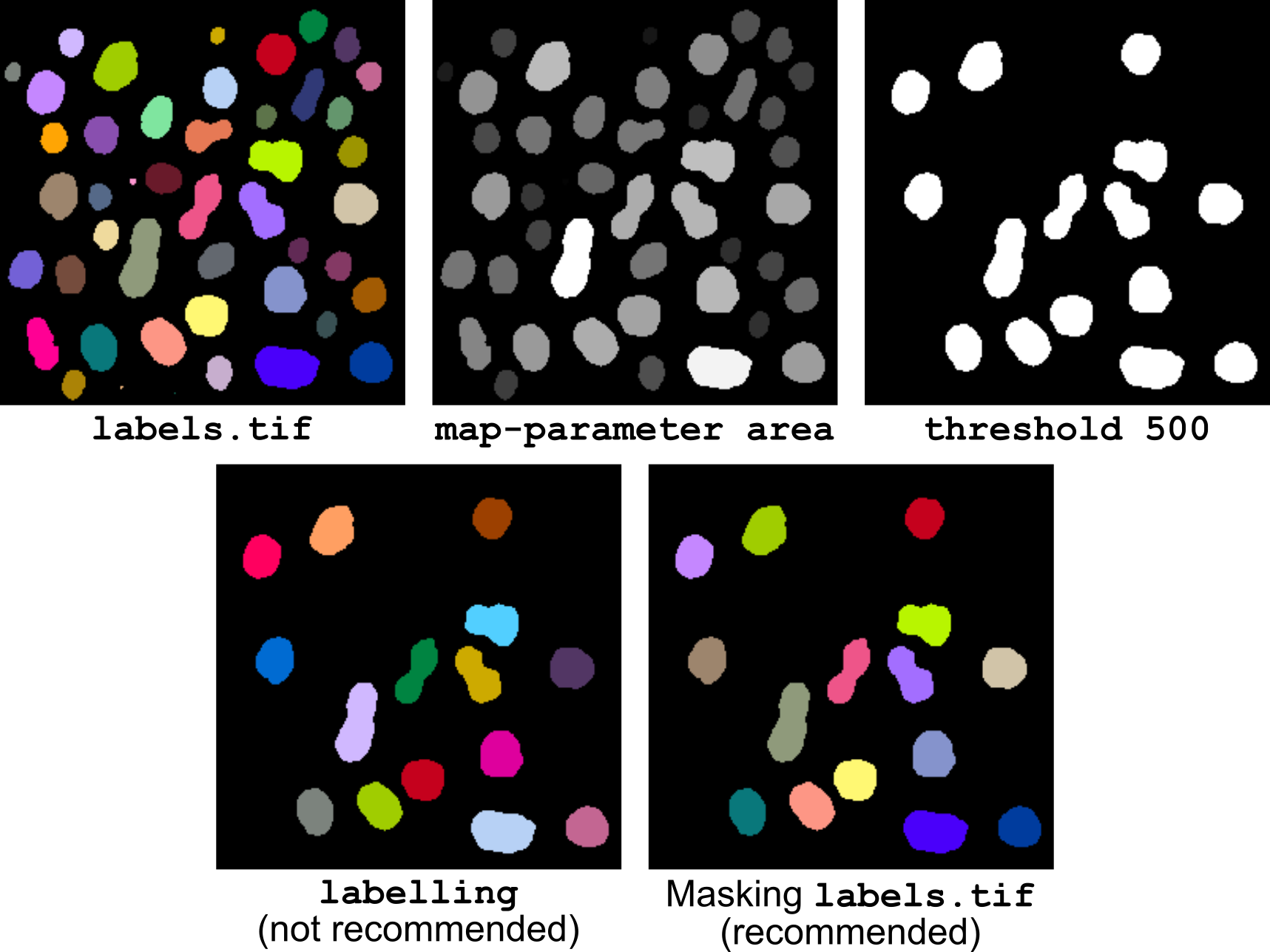
Figure 14 Selecting objects based on size.
Putting it all together into a single pipeline (illustrated in Figure 14) gives:
# keep a copy of labels for final masking
store $label-image

# threshold objects based on area
map-parameter area
threshold 500
store $binary-mask

# mask original labels with mask of selected objects
recall $label-image
mask $binary-mask
Selecting objects based on size and shape
Problem. This is a generalization of the problem of Selecting objects based on size: find the sequence of operations to remove in a segmented image all the objects that are below some size threshold (taking the number of pixels as a size measurement) and below an elongation threshold. Then write the corresponding pipeline file.
Answer. The principle is to first generate a map of object size and then threshold the map at the desired minimum size. Same is performed for elongation. The resulting two masks are used to filter in cascade the original label image (note they could also have been combined into a unique mask applied once to the labels):
bip map-parameter area labels.tif
bip map-parameter elongation labels.tif
bip threshold 500 labels-area.tif
bip threshold 1.5 labels-elongation.tif
bip mask labels-area-threshold.tif labels.tif
bip mask labels-elongation-threshold.tif labels-mask.tif
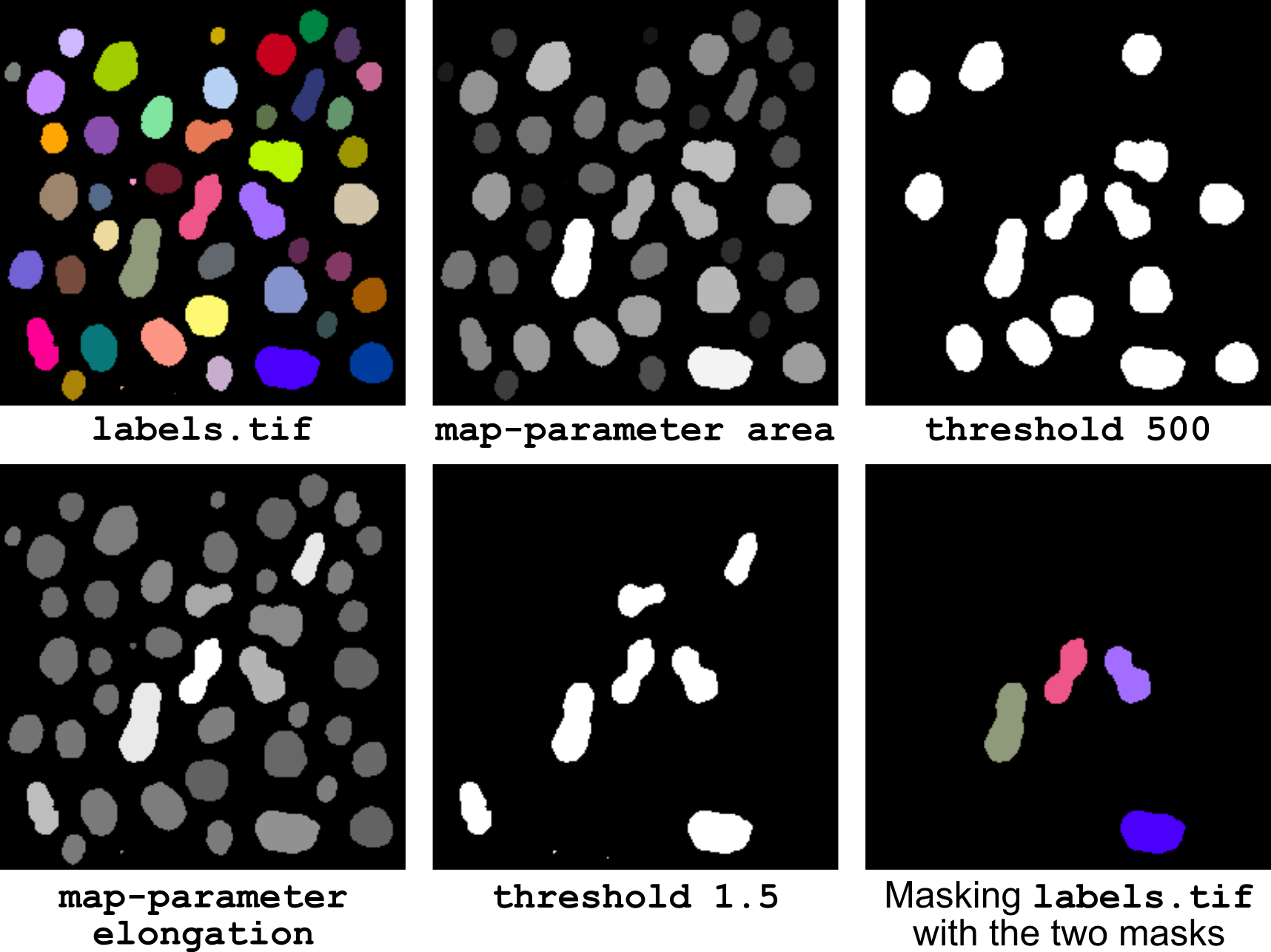
Figure 15 Selecting objects based on size and shape.
The corresponding pipeline (illustrated in Figure 15) is:
# keep a copy of labels for final masking
store $label-image

# threshold objects based on area
map-parameter area
threshold 500
store $area-mask

# threshold objects based on elongation
recall $label-image
map-parameter elongation
threshold 1.5
store $elongation-mask

# mask original labels with the two binary masks
recall $label-image
mask $area-mask
mask $elongation-mask
Labelling clusters of neighbouring objects
Problem. Starting from an image of labelled objects, find the sequence of operators that assigns a same label to objects that are close from each other (consider for example a distance below 5 units of physical distance). Then write the corresponding pipeline.
Answer. The principle is to dilate objects so that neighbours touch each other. The resulting aggregates are labelled and the original object shapes are recovered using masking by the input label image.
Note the dilation is performed below by thresholding the background distance map rather than by simply calling the dilation operator. This allows to handle images with non-cubic voxels (or non-square pixels), thanks to the --physical option of the Euclidean distance map operator (as done in the pipeline version below).
bip threshold 1 labels.tif
mv labels-threshold.tif tmp.tif
bip -f -b euclidean-distance --physical 0 tmp.tif
bip -f -b threshold 5 tmp.tif
bip -f -b invert auto tmp.tif
bip -f -b labelling tmp.tif
bip -f -b mask labels.tif tmp.tif
Tip: note how we repeatedly used a single intermediate image to store the successive steps in this sequence, thanks to the -f and -b options. This prevents generating multiple files with long filenames.
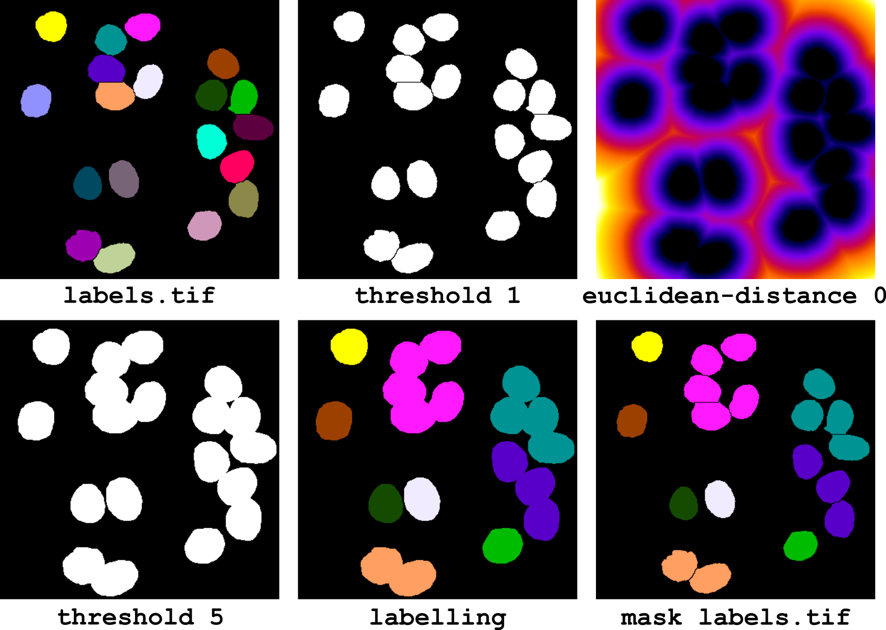
Figure 16 Labelling clusters of neighbouring objects.
The corresponding pipeline (illustrated in Figure 16) is the following:
# keep a copy of input labels
store $input

# dilate objects with R=5 physical units
threshold 1
euclidean-distance --physical 0
threshold 5
invert auto

# label clusters of objects
labelling

# recover original, individual object shapes
mask $input
Cell distance maps
Problem. Find the sequence of operators to compute the distance between each cell in a segmented tissue image to the innermost cells. Then write the corresponding pipeline.
Answer. Consider the innermost cells are the farthest ones from the cells at the periphery of the tissue. Therefore, the algorithm consists in first determining the innermost cells and then in computing the cell distance for each cell within the tissue to the inner core. This yields the following sequence of operations:
bip select-outer labels.tif
bip cell-distance labels-select-outer.tif labels.tif
bip select max labels-cell-distance.tif
bip -f cell-distance labels-cell-distance-select.tif labels.tif
Note the -f option in the last call: as this is the second call to the operator cell-distance on image labels.tif, there would be a conflict on output filenames. The -f option enforces overwriting existing files.
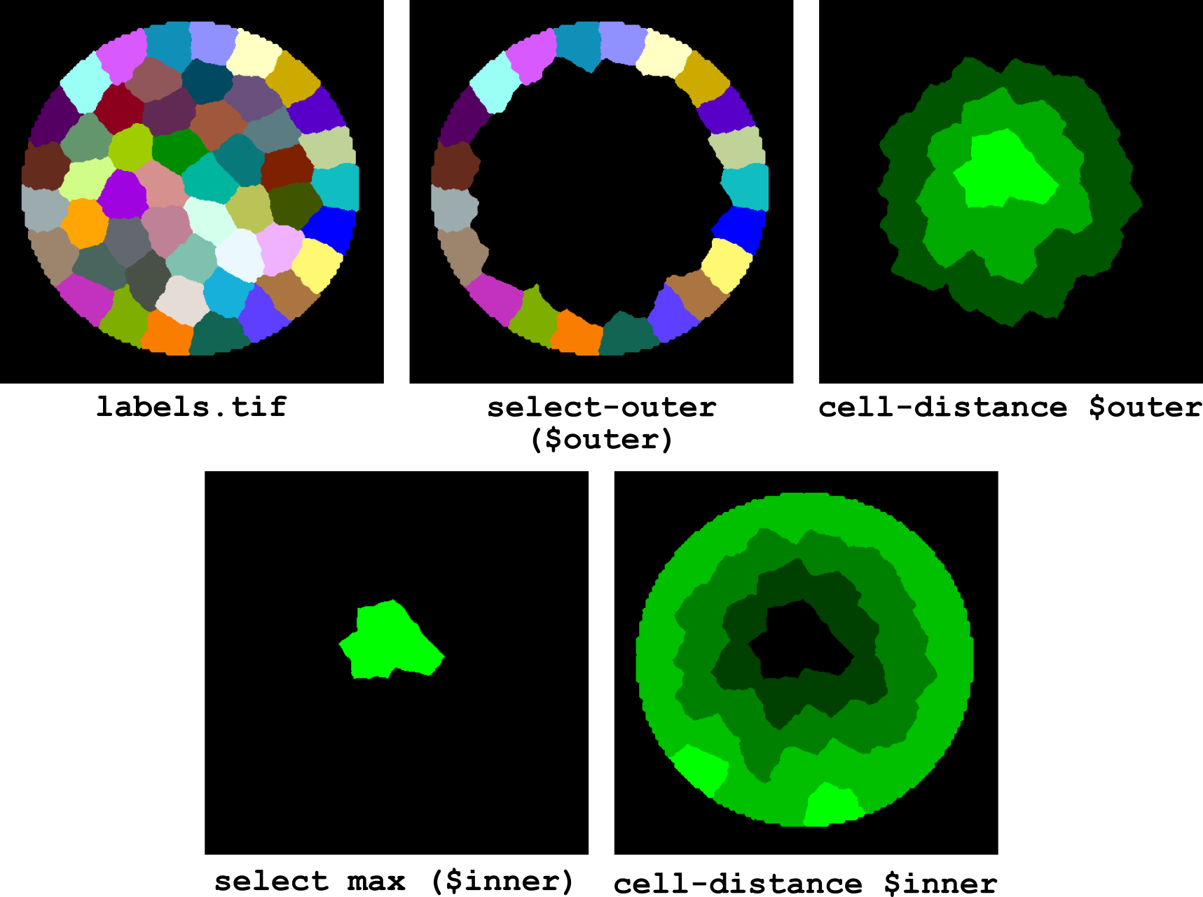
Figure 17 Computing cell distance from tissue center.
The corresponding pipeline (illustrated in Figure 17) is:
# make a copy of input labels
store $input

# select outer cells
select-outer
store $outer

# compute distance to outer cells
# and select the inner-most cells
recall $input
cell-distance $outer
select max
store $inner

# compute distance to inner cells
recall $input
cell-distance $inner